In general and specifically in clinical chemistry, a measurement is the process of determining the concentration of a biologically significant molecule in a biological fluid. The aim of all measurements is to obtain the true value. However, the result of the measurement will be only an estimate of the “true” value which remains unknown. We cannot know how near our measured value is to the “true” one.
This difference between the true and the measured value is the error, which can be random or systematic and whose true value is also unknown to us. When the systematic error (bias) has been accounted for, the remaining random error component is characterised by the measurement uncertainty or simply uncertainty, according to the “Guide to the expression of uncertainty in measurement” [1] (hereafter referred to as GUM). In the International vocabulary of metrology- Basic and general concepts and associated terms [2] (referred to as VIM), uncertainty is defined as “a non-negative parameter characterising the dispersion of the quantity values being attributed to a measurand, based on the information used” (paragraph 2.26). It defines an interval around the measured value, into which the true value lies with some probability. A measure of the uncertainty is the variance (the second central moment), although when talking about aggregate measurement uncertainty, other sources of uncertainty are often included. Often, the standard deviation (the square root of the variance) is reported instead, since it has the same units as the measured quantity.
Although the uncertainty characterises the error, it is not a difference between two values, does not have a sign (hence no direction)- unlike the error which does have a sign- and cannot be used to correct the result of the measurement. Although, both the true value and the error are abstract concepts whose exact values cannot be determined, they are nevertheless useful. Their estimates can be determined and are useful.
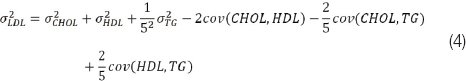
In clinical chemistry there are some parameters that are determined as a result of some calculation using other experimentally determined parameters [3]. A common one is the calculation of LDL using the Friedewald formula [4], from Total Cholesterol (CHOL), High Density Lipoprotein Cholesterol (HDL) and Triglycerides (TG):
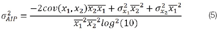
Another parameter calculated from the lipid profile is the Atherogenic Index of Plasma (AIP), which has been reported to be a good biomarker associated with cardiovascular risk [5-9] and is calculated as:
In this study, we examined the determination of the uncertainty of these calculated tests using various methods and compared them. We chose these two tests, because they are quite different in the calculation type. The first involved a linear relationship while the second involved the logarithm of a ratio.
Both LDL and AIP are calculated using other variables whose values have been experimentally determined and where each one has its own measurement uncertainty. In these cases, the challenge is to calculate the variance of these random variables, which are themselves a function of other random variables. This is called error propagation or propagation of uncertainty [10]. We used and compared different methods to calculate the mean and variance of LDL and AIP. We describe each of the methods, present and compare the results.
Materials and Methods
A total of four samples were used and CHOL, HDL and TG were measured 34 times once on each successive day on an ADVIA 1800 Chemistry Analyser by Siemens Healthineers. Each measurement was performed in duplicate and the mean was used. The samples had various combinations of low and high HDL and TG levels. The values of the measurements of the four samples are included in the [Table/Fig-1,2,3 and 4]. The mean, variance and CV of the CHOL, HDL and TG values for each of the four lipid measurement samples are shown in [Table/Fig-1]. Their empirical distributions are depicted as histograms in the supplement [Table/Fig-5,6 and 7]. The samples were created by pooling together patient samples so that desirable combinations of low and high parameter levels were created. The initial samples were anonymised. As a consequence of the method of creation of the pooled samples, they do not correspond to any individual. The pooled samples were aliquoted and the aliquots were frozen. A new aliquot was thawed each day in order to make the measurements.
Mean (mg/dL), variance (mg2/dL2) and CV (%), of the CHOL, HDL and TG values for each of the four lipid measurement samples.
| Parameter | Sample A | Sample B | Sample C | Sample D |
|---|
| Mean | Var | CV | Mean | Var | CV | Mean | Var | CV | Mean | Var | CV |
|---|
| CHOL | 290 | 67.2 | 2.8 | 200 | 41.8 | 3.2 | 259 | 38.8 | 2.4 | 147 | 20.1 | 3.1 |
| HDL | 56 | 67.2 | 14.5 | 61 | 91.8 | 15.7 | 76 | 120.8 | 14.5 | 33 | 43.2 | 19.9 |
| TG | 279 | 744 | 9.8 | 108 | 119.3 | 10.1 | 109 | 31.4 | 5.1 | 193 | 43.5 | 3.4 |
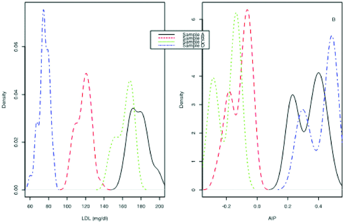
Distribution density of LDL (A) and AIP (B) for the four samples.
Corrrelation and covariance between (CHOL-HDL), (CHOL-TG) and (HDL-TG) for the four samples.
| Sample A | Sample B | Sample C | Sample D |
|---|
| Correlation between | Correlation | Covariance | Correlation | Covariance | Correlation | Covariance | Correlation | Covariance |
| Cor (CHOL, HDL) | -0.35 | -23.68 | 0.54 | 33.54 | 0.46 | 31.31 | 0.26 | 7.56 |
| Cor (CHOL, TG) | 0.64 | 143.93 | 0.66 | 46.62 | 0.12 | 4.11 | 0.26 | 7.8 |
| Cor (HDL, TG) | -0.59 | -132.24 | 0.23 | 23.73 | -0.58 | -36.03 | -0.72 | -13.34 |
*Pearson’s correlation coefficient
| Sample A | Sample B | Sample C | Sample D |
|---|
| LDL | | | | |
| Empirical distribution variance | 102.80 | 62.43 | 82.72 | 33.24 |
| Error propagation variance | 101.01 | 62.18 | 82.11 | 34.21 |
| Bootstrap variance median | 96.90 | 59.80 | 79.20 | 33.00 |
| Bootstrap variance 95 percentile | 58.7-141.8 | 38.0-87.4 | 51.0-107.4 | 18.8-50.3 |
| AIP | | | | |
| Empirical distribution variance | 0.00838 | 0.00477 | 0.00580 | 0.00883 |
| Error propagation variance | 0.00893 | 0.00520 | 0.00614 | 0.00957 |
| 2nd order error propagation variance | 0.00885 | 0.00517 | 0.00607 | 0.00958 |
| Bootstrap variance median | 0.00810 | 0.00460 | 0.00570 | 0.00860 |
| Bootstrap variance 95 percentile | 0.006-0.0102 | 0.003-0.0063 | 0.0042-0.0068 | 0.006-0.106 |
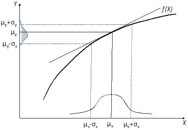
Mapping of a normal input distribution through a function. If the function f(X) is linear (diagonal line), the output distribution will be normal. If f(X) is non-linear (curved line), the output distribution may not be normal but skewed.
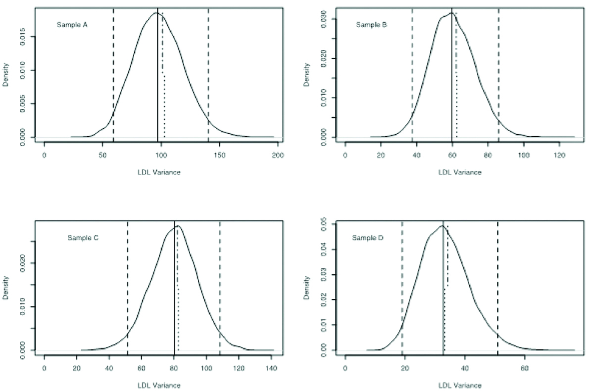
Distribution density of the bootstrap LDL variance. The median is shown as a continuous vertical line and the 2.5 and 97.5 percentiles as dashed vertical lines. The empirical variance is depicted as a dotted vertical segment from the bottom to the middle of the graph. The error propagation variance is depicted as a dash-dot vertical segment from the top to the middle.
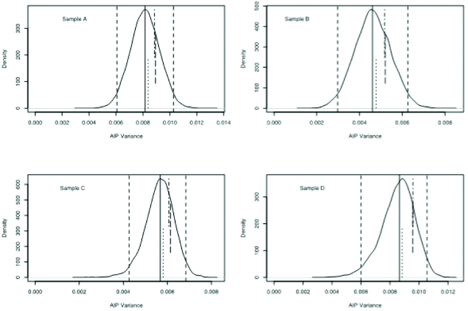
Distribution density of the bootstrap AIP variance. The median is shown as a continuous vertical line and the 2.5 and 97.5 percentiles as dashed vertical lines. The empirical variance is depicted as a dotted vertical segment from the bottom to the middle of the graph. The first order error propagation variance is depicted as a dash-dot vertical segment from the top to the middle and the second order error propagation variance as a dashed segment in the middle.
We can treat each clinical chemistry measurement as a random variable that follows a distribution. Although most clinical chemistry measurements have continuous values in an interval, since in practice they are determined and reported up to a small number of significant digits we can treat their distributions as discrete, which is what we have done in the rest of this study. It is of no practical interest if a glucose value is 100.0 or 100.1 or if a calcium value is 9.53 or 9.54.
All analyses and calculations were performed in the R programming language [11]. The whole analysis (R code, figures and tables included in the article as well as other figures and tables not included in the main text) is available as supplemental material.
To derive the formulas for the variance of LDL and AIP using error propagation, we used the general formula of the uncertainty for correlated input variables in the GUM section 5.2, equation (13).
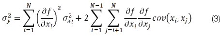
where xi and xj are the expected values of the random variables Xi and Xj, σ2 is the variance of the subscripted variable and cov(xi, xj) is the estimated covariance associated with xi and xj.
For LDL, if we set x1=CHOL, x2=HDL and x3=TG, the partial derivatives are, ∂LDL/∂CHOL=1, 2202LDL/∂HDL=-1 and ∂LDL/∂TG=-1/5. Substituting in equation (3) we get:
For AIP, if we set x1=TG and x2=HDL, the partial derivatives are ∂AIP/∂TG=1/TGln10 and ∂AIP/∂HDL=-1/HDLln10 and the equation for the AIP variance is:
where is the expected value of the subscripted variable.
Note that for AIP, TG and HDL must be expressed in mmol/lt. If expressed in mg/dL, TG must be multiplied by 0.0113 and HDL by 0.0259.
The above equations (4) and (5) that stem from the general form (3) are derived according to [12] (section 5.5.4). The derivation involves an approximation using the first-order Taylor expansion of the mapping function f(). This approximation is sufficient when f() is linear or approximately linear in the interval, as is the case for LDL. However, in the case of AIP that involves a log ratio (and also in cases of other highly non-linear functions) this approximation will not hold, as shown in the Results section. We determined the variance using the method of [12], but taking into account the second-order Taylor series term also. The formula for the variance of AIP (given x1=TG, x2=HDL) that resulted is:
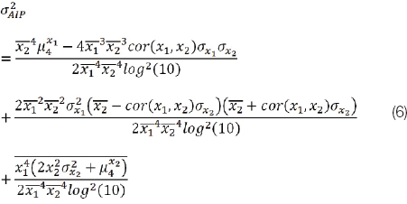
where, μ4xi is the fourth central moment of the subscripted variable and cor(x1, x2) is the correlation coefficient between x1 and x2 and again x1=TG and x2=HDL.
Results
Normality of the Data
A common but often erroneous assumption made by clinical chemists is that repeated measurements will give an (approximately) normal distribution. Moreover, an assumption made in error propagation is that the distribution of the output quantity is normal or t-distributed. However, as it is known, this is not always the case. We created the histograms of our input quantities (CHOL, HDL and TG) and output quantities (LDL and AIP), to check if they are (at least nearly) normal. For the input quantities CHOL, HDL and TG it is evident from the supplemental figures 1-3 that they are not normally distributed. Also, as shown in [Table/Fig-2], the density of both LDL and AIP for all four samples is far from normality. In fact all of them are multimodal. It should be noted that the distributions depicted in [Table/Fig-2] would be more correct to have been presented as histograms and not densities. However, the density approximation depiction is more illustrative and this is the reason it was chosen.
Correlation of Parameters
An assumption often made when dealing with multiple random variables is that they are independent and uncorrelated. In the case of CHOL, HDL and TG, even if they are independent it is certainly possible that they are correlated. Even if the determination reactions are independent, there are underlying common biological processes that affect the levels of many lipids. We determined Pearson’s correlation coefficient and the covariance for the pairs (CHOL-HDL), (CHOL-TG) and (HDL-TG) for the four samples, presented in [Table/Fig-3]. From the correlation coefficients we can conclude that in many cases there is a significant correlation (e.g. HDL-TG) and in other cases the correlation is weaker (e.g sample CHOL-TG). Also, in the supplement figures 5-7 the scatterplots of the pairs of the parameters are shown along with the linear regression lines. We can see that in most cases the parameters cluster in two groups: one in which there does not seem to be any correlation and a smaller cluster of potential outliers which appears to affect the whole correlation.
In the GUM (and measurement theory in general) a distinction is made when the quantities are independent (section 5.1-Uncorrelated input quantities) and when they are correlated (section 5.2 - Correlated input quantities). As stated, the former case is “valid only if the input quantities Xi are independent or uncorrelated... If some of the Xi are significantly correlated, the correlations must be taken into account”. Since in this case the quantities seem to be correlated (even if they may be independent), it would be prudent not to make assumptions of no correlation and use instead the joint probability distribution function for error propagation.
Variance using the Empirical Distribution
The most simple and obvious method to determine the variance of a calculated test would be to use the empirical distribution. In this case we would measure the experimentally measured quantities (CHOL, HDL and TG in this case) and use them to determine the calculated quantities (LDL and AIP). Then we would use these values to calculate the variance. This empirical distribution variance for the four samples for both LDL and AIP is shown in [Table/Fig-4] (first row of the LDL and AIP section of the table).
The reason this is not the correct approach is explained in [13] and shown in [Table/Fig-5]. When we have one or more random input variables (e.g., CHOL, HDL, TG) each one with its own distribution and a function f() of these variables (e.g., a formula for the calculation of LDL or AIP), then the output is a random variable with its own distribution (e.g., LDL or AIP). As shown in [Table/Fig-5] and [13], when the input distribution is mapped through a non-linear function, the output distribution may be skewed. When this happens the empirical approach (which assumes a normal output distribution) is not the best approach.
Variance using Error Propagation
Another approach (that is in essence the same to the first one), is to use error propagation or propagation of uncertainty [10,13]. We also calculated the variance of LDL using error propagation. This approach may work well enough if the function is approximately linear in the interval, where it is the expected value and standard deviation of the input variable, as shown in [Table/Fig-5]. The error propagation variance of LDL and AIP are shown in [Table/Fig-4].
We can see that for LDL the empirical and error propagation variances are nearly the same, with the small differences (from ~0-3% absolute value of the relative difference) being easily attributable to rounding errors and approximations always present when calculating floating point numbers in a digital computer. However, in the case of AIP (whose function is non-linear), the absolute values of the relative difference is from ~6-9%, which results from the inaccurate approximation of this function using only the first-order Taylor series. When we calculated the second-order Taylor approximation things changed very little. Evidently, the use of Taylor series in the case of the log function is insufficient unless many more terms are included, which is very difficult given the complexity of the formula even for a first-order (equation 4), much more for the second-order approximation (equation 5). In the supplement Figure 9 the linear form for the equation of LDL is depicted graphically and in supplement figure 10 the non-linearity of AIP is depicted.
Variance using Bootstrapping
Another method we used to determine the variance is bootstrapping (random sampling with replacement) [14-15]. In this method, the experimental distribution is used and not a parametric one from which samples are drawn, as in Monte Carlo simulation. In contrast to Monte Carlo, the data is used as given, with no assumptions made about the distribution.
A number of samples (in this case 20) were drawn with replacement from the joint empirical distribution of the triples of {CHOL, HDL and TG} values. This procedure was repeated to get 2000 realisations and for each realisation the variance of LDL and AIP was calculated. Aggregate statistics on the ensemble were then computed. In [Table/Fig-6,7], the distribution density of the bootstrapped variances of LDL and AIP, respectively, are shown, with the empirical and error propagation variances depicted as vertical segments. Also, in [Table/Fig-4], the numerical values for the LDL and AIP variances are shown. It is evident that the median bootstrap variances are lower than the empirical and error propagation ones, especially for AIP.
Variance of Output Variable when the Variances of the Input Variables Change
To see if this discrepancy between methods occurs not only for these specific samples and to determine its behavior in general, we determined the variance of LDL and AIP using both the error propagation formula(s) and bootstrapping using a series of distributions with increasing variance of CHOL, HDL and TG (one at a time) while keeping the mean constant. A series of distributions of increasing variance and constant mean were created. The mean was kept equal to the mean of each sample. For each distribution with increasing variance of CHOL, HDL and TG (separately), the LDL and AIP variances were calculated using the empirical, error propagation and bootstrap approaches. In total 20 plots were generated (12 for LDL, four samples by 3 variances each and 8 for AIP, four samples by 2 variances each). In [Table/Fig-8], some representative plots are shown. All the plots can be seen in the supplement figures 16-20.
Plot of LDL [(A)-(C)] and AIP [(D)-(F)] empirical, error propagation and bootstrap variance versus increasing variance of CHOL, HDL or TG, as indicated in the abscissa for differing samples (indicated in each sub-figure).
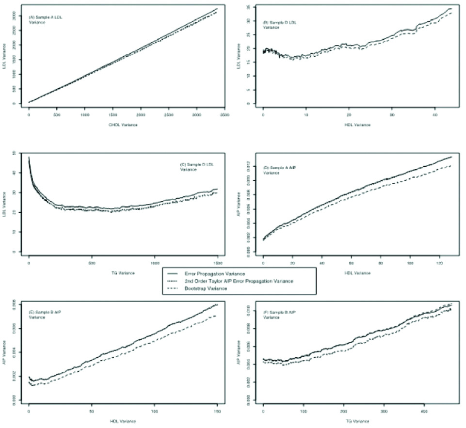
It is evident that there is a large variation of the behaviour of the LDL and AIP variances as the variance of either CHOL, HDL or TG changes. Some curves are linear and others not. There are however, three common themes in all plots. The bootstrap variance is lower than the error propagation variance, for AIP the 2nd order error propagation variance is very near the first order one and all the variances fluctuate in tandem.
Discussion
All measurements have an inherent uncertainty, quantified here by the variance. In clinical chemistry there is a variety of approaches to determine the measurement uncertainty [16,17].
In the case of calculated clinical chemistry tests, we must take into account the propagation of the uncertainty of multiple parameters into the final result. There are three main methods to deal with this fact: The first is the empirical/theoretical (using error propagation) approach. We bundle the empirical and error propagation methods together, since they both use the same function to map the distribution of one or more random input variables to the distribution of a random output variable. The second is using Monte-Carlo sampling and the third is by bootstrapping. All three methods have their advantages and weaknesses:
The empirical/theoretical approach has a rigorous mathematical background, however certain assumptions must be met, namely
The errors in each variable be uncorrelated. If correlated, a joint probability distribution function for all the variables must be derived.
The probability distribution function for the output variable be normal or nearly normal.
Linearisation of the mapping function result in an adequate approximation.
The Monte Carlo simulation is more robust, but
It also suffers from the fact that a parametric form of a probability distribution function describing the data must be used, while in fact the data may not follow any such function.
Can be computationally expensive.
Finally, the bootstrap approach makes no assumptions about the distribution of the data or the errors, but uses instead the empirical distribution and not a parametric one. Some of its drawbacks are that it
Can fail when the distribution does not have finite moments (not an issue in clinical chemistry),
Is not well suited to small sample sizes,
Can fail when large samples relative to the population size are used and
Is computationally expensive.
In this study, we used both error propagation and bootstrapping to estimate the uncertainty of LDL and AIP as calculated from measurements of CHOL, HDL and TG. A total of four samples were used with various combinations of CHOL, HDL and TG levels.
In the case of lipid profile tests, we cannot assume that the parameters measured are either independent or uncorrelated, which was the case with our data. Therefore, in the error propagation approach a joint probability distribution for all parameters was used to derive the variance. This is essentially the case in equation [3].
Another assumption in error propagation is that the input variables are normal. In the supplement figures 1-3 the distribution of the input variables CHOL, HDL and TG are shown and they are not normal. Also, neither the distribution of the output variable (in our case LDL and AIP) is normal. In [Table/Fig-2], it is evident that the distributions of LDL and AIP for all four samples are neither normal, nor do they follow some closed-form distribution. In fact, all of them are multimodal.
In Supplement 1 to the GUM an alternative to the GUM framework for uncertainty evaluation is described, which does not use error propagation theory, but a Monte Carlo approach and does not assume a normal or t- distribution [18]. This approach however, suffers from the drawback that a probability distribution function must be assigned to the data, using either a Bayesian approach [19] or the principle of maximum entropy [20]. This assigned distribution can take a number of forms, from a vague one (e.g., rectangular, curvilinear trapezoid and more) to more defined ones (e.g., exponential, gamma or other). This approach, although superior to the error propagation method (when its assumptions are not met), must also approximate the empirical distribution with a parametric one. This can be especially problematic when the empirical distribution is not unimodal (as is the case for LDL and AIP in this study). For this reason we did not use Monte-Carlo simulations in this study. There is of course the possibility that if more measurements were made, the distribution would approach normality, but this is an assumption that cannot be made beforehand, plus the fact that a large number of measurements would probably have to be taken.
On the other hand, the bootstrap approach does not make any assumptions about the empirical distribution nor does it assign a distribution function to it. This is demonstrated in Supplemental figure 21, where the consequence of the central limit theorem is depicted for the LDL values of sample A. As we average a larger sample of data points from the empirical distribution and create the distribution of the resulting averages, this distribution approaches the normal one.
In the case of LDL and AIP it seems that the empirical/theoretical approach overestimates the uncertainty. This is less pronounced for LDL, where the function is linear and more pronounced for AIP with a non-linear function. Also, the use of second order Taylor approximation does not seem to improve things significantly, whereas it increases the complexity disproportionately to the improvement it confers. The use of higher order Taylor approximation would be impractical, especially in cases where we must take into account the correlation of the input variables. The resulting formulas would be too complex to be useful.
Finally, it would also be interesting to study calculated tests of other parameters, not related to the lipid profile, like e.g., creatinine clearance [21,22].
Limitation(s)
It should be stated here that the use of the GUM, partial derivatives, bootstrapping and Taylor series, although normal for statisticians, may be too much for many well-intentioned clinical chemistry practitioners. However, their use is not necessary in the majority of clinical chemistry tests. Most of them can be performed without loss of accuracy by variance component analysis and simple addition of variances without partial derivatives and Taylor expansion. The more complicated approach presented in this paper is required only when functions based on a number of different parameters are performed including the LDL and especially the AIP. However, in these cases it can be very useful.
Conclusion(s)
We can therefore conclude that for calculated tests it would be more appropriate to use the bootstrap approach, especially in non-linear functions like AIP, since the error propagation approach would overestimate the measurement uncertainty. In such highly non-linear functions even if the input variable is normal (which may very well not be) the output variable will not be normal and therefore the assumptions made for empirical calculations do not hold. Another reason to use bootstrapping is that we can get not only some numbers describing a distribution (e.g., mean and standard deviation), but the entire distribution of values, which is useful when the distribution is not a parametric one, as is the case here. The proper way to describe a distribution that does not have a closed form is to give the entire distribution.
*Pearson’s correlation coefficient