Introduction
A cross tabulation is often used while analysing a categorical variable in which the frequency of each possible combination are noted. Contingency table is a table of joint count for various combinations of categories of the two cross-classified categorical variable. The order of a contingency table, R×C, indicates the number of levels of the two categorical variables in consideration. When the response is categorical, the data fits a contingency table in two ways viz., unrestricted sampling and restricted sampling with fixed total sample size. In a restricted sampling scheme, it is assumed that the marginal or grand total is fixed. This sampling scheme is also referred as a binomial or multinomial sampling scheme. The unrestricted sampling scheme is also referred as a Poisson sampling scheme. We often assume that data has been generated from Poisson, binomial or multinomial sampling schemes [1]. All the three sampling schemes lead to the same estimated expected cell values [2]. In the present paper; the analysis of contingency tables generated using categorical data from a complex sampling scheme is discussed. A complex sampling scheme constitutes the data comprising between-observation dependence which makes the multinomial sampling scheme invalid. These departures from multinomial sampling affect Pearson’s chi-squared statistic and hence makes this test not suitable to be used in case there exists between observation dependence [3]. A categorical variable has a measurement scale consisting of a set of categories [1], assigning each individual to a particular group based on some qualitative property. Categorical data are the counts corresponding to a set of non-overlapping classes of a qualitative variable. Categorical scales are pervasive in the biomedical sciences to measure outcomes such as whether a treatment is successful or not [1].
The analysis of data collected depends on the measurement scale. The measurement scale is nominal if the categories are meant just for identification such as “males or females.” A variable is said to be measured on the ordinal scale if the categories exhibit a natural ordering, for example, severity of disease with categories “mild”, “moderate” and “severe.” Comparison of independent samples includes the variability in response along with the variability between subjects. However, when the data are paired, we look at the data within each subject. The paired comparison is not affected by the way subjects differ [4], ruling-out the possibility of between-subject variability. It is observed that the researcher use chi-square test of association or Fisher’s exact test [5] on paired data, which is not appropriate because these tests treat each observation as independent to each other. If a paired study is undertaken, a paired analysis must be used [6]. In this paper, we discuss in detail, the tests suitable to deal with paired nominal data.
Categorical Data Analysis
McNemar’s Test
The McNemar’s test is used on paired nominal data. This test is often used to test marginal homogeneity. Marginal homogeneity is said to hold if the row and corresponding column marginal frequencies are equal. This test applies to studies where cases serve as their control, or in studies with “before and after” design specifically when the variable of interest is dichotomous [4]. In such situations, one cannot apply any parametric tests since the parametric tests require the variable to be measured at-least in interval scale.
Consider a dichotomous variable measured at two different time points. The researcher is interested to investigate if there is any change in the response over time. A 2×2 contingency table for this is as illustrated in [Table/Fig-1].
Data layout for McNemar’s test.
| Time point 2 |
|---|
| | Level A | Level B | Total |
|---|
| Time point 1 | Level A | a | b | a+b |
| Level B | c | d | c+d |
| Total | a+c | b+d | n=a+b+c+d |
The cells with count a and d are called as concordant cells as they represent individuals with no change in the status of response over time [4]. As the cell counts b and c indicate the change in the response over time, they are known as discordant cells. We hypothesize that there is a significant change in the response at two time points. There is significant difference in the proportion of individual with response A in the first and B in second-time point to the proportion of individual with response B in first and A in second time point i.e., πAB≠πBA. This can be simplified to πA+≠π+A, which implies that marginal proportions are not equal. Thus, the hypothesis can be revised as the proportion of individual with response A at first time point does not differ significantly to the proportion of individual with that at the second time point. The hypothesis mentioned is known as the hypothesis of marginal homogeneity [7].

The test statistic follows the chi-squared distribution with 1 degree of freedom under the null hypothesis of no change.
Case 1: A program to create awareness on the side effect of smoking was conducted among college students, at a regular interval of three months. Three contact programs were organised. The data on smoking status and other socio-demographic profile was collected at baseline and after completion of the program. We hypothesize that the intervention was effective. The aggregated data is illustrated in [Table/Fig-2].
Setup for the study requiring a binary categorical response at two time point on the same set of individual.
| After 3 months |
|---|
| | Smokers | Non-smokers | Total |
|---|
| Baseline | Smokers | 70 | 130 | 200 |
| Non-smokers | 30 | 154 | 184 |
| Total | 100 | 284 | 384 |
The McNemar’s test statistic is calculated as 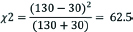 . A significant difference in the proportion of smokers after three months was observed (χ2=62.5, df=1, p<0.001). There is enough evidence to conclude that the awareness program was effective. [Table/Fig-3] summarises the McNemar’s test.
Summary of McNemar’s test.
| General | Case 1 |
|---|
| Hypothesis | There is significant difference in the proportion of individual with response A in the first and B in second time point to the proportion of individual with response B in first and A in second time point | There is significant difference in the proportion of smokers at baseline to proportion of smokers at three months |
| Test statistic |  | χ2=62.5, p<0.001 |
| Decision rule | If  or p≤0.05 Reject H0 or p≤0.05 Reject H0 |  , p≤0.05 Reject H0 , p≤0.05 Reject H0 |
Points to Ponder: McNemar’s test was used since the importance was given to baseline and the last time point observation. In case we wish to investigate the change in smoking status at each time point (contact program 1, 2 and 3) we would rather use Cochran’s Q test. A major limitation of McNemar’s test is that it cannot be used if the variable of interest has more than two levels or is measured at more than two time points. In such situations, one should utilise alternative tests like Stuart Maxwell test or Cochran Mantel Haenszel correlation test as discussed in this paper.
In Case 1, suppose the variable smoking status has more than two levels say non-smokers, 1-10 cigarettes per day and more than ten cigarettes per day. With the said modification in the response levels, McNemar’s test cannot be applied to test for marginal homogeneity.
Stuart Maxwell McNemar’s Test of Marginal Homogeneity
Stuart Maxwell McNemar’s test is an extension to McNemar’s test when there are two dependent samples and the response has three or more categories [8]. If the variable of interest has I categories and is put in a contingency table, then an I×I will be generated. Here we hypothesize that,  . The data layout is shown in [Table/Fig-4].
Data layout for Stuart Maxwell McNemar’s test.
| Time point 2 |
|---|
| Level 1 | Level 2 | … | Level n | Total |
|---|
| Time point 1 | Level 1 | n11 | n12 | | n1n | n1+ |
| Level 2 | n21 | n22 | | n2n | n2+ |
| ... | ... | ... | | ... | ... |
| Level n | nn1 | nn2 | | nnn | nn+ |
| Total | n+1 | n+2 | | n+n | n++ |
The Stuart Maxwell McNemar’s test statistic,
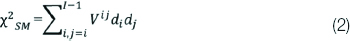
The test statistic follows chi-squared distribution with (I–1) degrees of freedom. Where, Vij is the variance covariance matrix [9],  is difference in corresponding marginal total [7].
Case 2: Let us consider the smoking status has three categories say non-smokers, 1–10 cigarettes per day and >10 cigarettes per day. The aggregated data is illustrated in [Table/Fig-5].
Setup for the study requiring a multinomial categorical response at two time point on the same set of individual.
| After 3 months |
|---|
| | Non-smokers | 1-10 cigarettes per day | >10 cigarettes per day | Total |
|---|
| Baseline | non-smokers | 45 | 37 | 28 | 110 |
| 1-10 cigarettes per day | 55 | 32 | 11 | 98 |
| >10 cigarettes per day | 105 | 18 | 53 | 176 |
| Total | 205 | 87 | 92 | 384 |
The Stuart Maxwell McNemar’s test statistic  indicates enough evidence to reject the null hypothesis and conclude that the intervention was effective in creating awareness among college students. [Table/Fig-6] summarises the Stuart Maxwell McNemar’s test.
Summary of Stuart Maxwell McNemar’s test.
| General | Case 2 |
|---|
| Hypothesis | There is no marginal homogeneity. | There is significant difference in the proportion of smoker at baseline to proportion of subjects at 3 months |
| Test statistic |  | 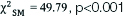 , p<0.001 , p<0.001 |
| Decision rule | If  or p≤0.05 Reject H0 or p≤0.05 Reject H0 |  , p≤0.05 Reject H0 , p≤0.05 Reject H0 |
Points to Ponder: Stuart Maxwell McNemar’s test is suitable only if we have a square table. It is suggested not to use this test when the response is measured at more than two time points. It can’t be either used in situations where k(>2) interventions are given to the same individual. Instead, we need to use Cochran Mantel Hanszel Correlation test in the above-mentioned situations.
Let’s suppose that in Case 1, the smoking status was recorded at more than two-time points. McNemar’s test is not suitable for a situation where a dichotomous response is observed at more than two time points.
Cochran’s Q Test
Cochran’s Q is a test for analysing data on three or more dependent samples where the response variable is binary [8,10]. It is an extension of McNemar’s test for related samples and provides a method for testing the differences between three or more matched sets or three or more time points. The test can also be used to compare two or more interventions on the same set of an individual with sufficient washout time ensuring no carryover effect of the previous intervention. In such case, each subject is treated as a block. Suppose a binary response is measured at K time points on individuals where each individualis a block. The data layout is shown in [Table/Fig-7].
Data layout for Cochran’s Q test.
| Subjects | Time Point |
|---|
| 1 | 2 | … | K |
|---|
| 1 | X11 | X12 | ... | X1k |
| 2 | X21 | X22 | ... | X2k |
| 3 | X31 | X32 | ... | X3k |
| … | ... | ... | ... | ... |
| B | Xb1 | Xb2 | ... | Xbk |
In such case, we are interested in testing if the proportion of response Xij is the same at each time point. Here Xij is the categorical response corresponding to the ith subject at the jth time point. Each Xij take values either 0 or 1 where 0 implies non-occurrence and 1 implies the occurrence of the event. Then, X+j represents the sum for the jth column and Xi+ represent the sum for the ith row (individual). Let N be the total number of success.

The test statistic follows a chi-squared distribution with k–1 degrees of freedom under the null hypothesis of no change.
Case 3: Let us consider a modification in case 1. The smoking status was measured at three time points say baseline, one year and after two years. The table set up is given in [Table/Fig-8].
Table setup for the study requiring a binary categorical response at multiple timepoint on same set of individual.
| Subject | Baseline | After 1 year | After 2 years |
|---|
| 1 | 1 | 1 | 0 |
| 2 | 0 | 1 | 0 |
| 3 | 0 | 1 | 0 |
| 4 | 0 | 1 | 0 |
| 5 | 1 | 1 | 0 |
| 6 | 0 | 0 | 1 |
| 7 | 1 | 0 | 1 |
| 8 | 1 | 0 | 1 |
| 9 | 0 | 0 | 0 |
| 10 | 0 | 1 | 0 |
In this case, we hypothesize that the proportion of smokers decrease significantly over time where, K=3, b=10, X+1=4, X+2=6, X+3=3, X1+=2, X2+=1, X3+=1....X10+=1 and N=13. The test statistic T=1.55, df=2, p=0.459, which indicates no enough evidence to reject the null hypothesis. The intervention is not effective in reducing the number of smokers over time. [Table/Fig-9] summarises the Cochran’s Q test.
Summary of Cochran’s Q test.
| General | Case 3 |
|---|
| Hypothesis | Proportion of success differs significantly for at least one group (time point) | Proportion of smokers differs significantly for at least one time point. |
| Test statistic | 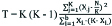 | T=1.55, p=0.459 |
| Decision rule | If  or p≤0.05Reject H0 or p≤0.05Reject H0 |  , p>0.05Not enough evidence to reject H0 , p>0.05Not enough evidence to reject H0 |
Points to Ponder: Cochran Q test is equivalent to McNemar test when K=2 [8]. For a similar design with an ordinal or continuous response, one instead uses the Friedman’s test. The case where there are exactly two treatments the test is equivalent to McNemar’s test. Post-hoc for Cochran’s Q is McNemar’s test for each pair, using Bonferroni-Dunn method of correction [8].
Cochran Mantel Haenszel (CMH) correlation test: This method is used when we have paired nominal data with more than two levels measured at more than two time points. McNemar’s test and Stuart Maxwell McNemar’s test are the special cases of CMH correlation [11]. Each subject is treated as a stratum. Within strata, number of rows represents time points, and columns represent categories of response [12]. For kth subject, the partial table is represented in [Table/Fig-10].
kth Stratum data Layout for CMH Correlation test.
| Response category |
|---|
| Time Point | 1 | 2 …………………………………C | Total |
|---|
| 1 | nk11 | nk12……………………………….. nk1C | 1 |
| 2 | nk21 | nk22……………………………….. nk2C | 1 |
| . | . | . | . |
| . | . | . | . |
| T | nkT1 | nkT2……………………………….. nkTC | 1 |
| Total | nk+1 | nk+2 ………………………………..nk+c | T |
Nij, where i=1,2,...,T, j=1,2,...,C, may take value either 0 or 1 depending on the status of the kth subject at a particular time point such that row sum is equal to one. Thus, if we have n subjects, we will have n such partial tables. To test the conditional independence (two variables are said to be conditionally independent if they are independent in each partial table), CMH test statistic is used.
For an ixjxk table, the CMH test statistic is given by,

The test statistic follows chi-squared distribution with (T–1)x(C–1) degrees of freedom [13]. In the kth stratum,  . Each nk is the vector of (T–1)×(C–1) cell counts, μk is the vector of expected frequencies of (T–1)x(C–1) cells, and Vk is the variance covariance matrix where. ∂ab = 0 if a ≠ b and ∂ab=1 if a=b. The equation (5) gives the variance covariance matrix.

Case 4: Let us consider a modification in case 1, where smoking status has three levels as discussed in case 2 (non-smokers, 1-10 cigarettes per day and >10 cigarettes per day) and is measured at more than 2 time points as in case 3 (baseline, after three months and after six months). Table setup for the ith subject is given in [Table/Fig-11].
Table setup for the study requiring multinomial categorical response at three time points on kth individual.
| Response category |
|---|
| Non-smoker | 1-10 cigarettes per day | >10 cigarettes per day | Total |
|---|
| Baseline | 0 | 0 | 1 | 1 |
| After 3 months | 0 | 1 | 0 | 1 |
| After 6 months | 0 | 1 | 0 | 1 |
Data for all 384 subjects were analysed using the SAS University edition. The evidences were not enough to reject the null hypothesis (χ2=0.189, df=4, p=0.909). The intervention is not effective in reducing the number of smokers over time. The results for CMH correlation test is summarised in [Table/Fig-12].
Summary of CMH correlation test.
| General | Case 4 |
|---|
| Hypothesis | There is a linear association between X and Y in at least one stratum. | Proportion of smokers differs significantly for at least one time point. |
| Test statistic |  | χ2 = 0.1893, p=0.909 |
| Decision rule | If 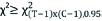 or p ≤ 0.05Reject H0 or p ≤ 0.05Reject H0 |  , p>0.05Not enough evidence to reject H0 , p>0.05Not enough evidence to reject H0 |
Points to Ponder: When the response is binary and is measured at more than two time points, we instead use Cochran’s Q test. When the response has more than two levels, measured at two time points, we use Stuart Maxwell McNemar’s test. When response is binary and is measures at two time points, we use McNemar’s test instead.
A tabular comparison to summarise the situation and the appropriate choice of the test is shown in the [Table/Fig-13].
Comparison of tests discussed in the article.
| Test | Situation |
|---|
| McNemar’s | Response levels: 2Time points: 2 |
| Stuart Maxwell McNemar’s | Response levels: >2Time points: 2 |
| Cochran’s Q | Response levels: 2Time points: >2 |
| Cochran Mantel Haenszel | Response levels: >2Time points: >2 |
Conclusion
The statistical test to be used on the paired data depends on the number of levels of categorical response and the number of time point (s) measurement is taken. Use of independent sample techniques on paired data results in loss of information and unreliable results. Therefore, it is recommended to study the characteristics before deciding on the statistical tests suitable for the data collected.