Obesity as a disease has become an epidemic, not only in the developed world but in developing countries as well. It is a major public health problem due to its connection with increased morbidity and reduced quality of life [1,2]. Obesity is linked with many types of cardiometabolic disturbances and metabolic syndrome [3]. It is now labeled by the World Health Organization as one of the most serious public health problems of the 21st century [4]. A precise analysis of body composition is imperative to recognise health risks associated with excessive body fat, observe changes in body composition linked with certain diseases, as a support to developing weight loss or weight gain programs and assessing the success of nutrition and exercise interventions, and to supervise age-related changes in body composition.
BMI is generally used to categorise obesity; although, it is a very crude measure of obesity, as it does not distinguish between tissues like muscle and fat [5]. Standard BMI cut off values may not be suitable to use in the elderly population due to age-related changes in body composition [6,7] like there is progressive loss of muscle mass and increase in fat mass [8,9]. For diagnosis of obesity, it is imperative to measure only the fat compartment of the body and this is best done by the measurement of visceral and subcutaneous fat. Magnetic Resonance Imaging (MRI) and Computed Tomography (CT) are the reference methods for estimating visceral and subcutaneous fat quantities and distribution, the use of which in large scale studies is often restricted by their costs, convenience and due to radiation exposure [10]. Abdominal USG can easily be used to obtain an indirect one-dimensional estimate of the fat component and has been validated against MRI and CT as a way of estimating the visceral and subcutaneous fat distribution in large scale studies [11]. In contrast to the disadvantages of CT, MRI and anthropometric measurements, USG has shown to be a simple, cost-effective method without radiation risk, and with already proven reproducibility and reliability [12-14]. USG has been used competently to evaluate body fat since time immemorial; however, this technique has not been employed as a body composition technique. This is because many students, researchers, and clinicians are unfamiliar with its usefulness and versatility as a body composition assessment tool [15]. Therefore, this study was carried out with an aim to establish the role of USG as a quantitative measure of obesity by measurement of SAFT and ST.
Materials and Methods
This prospective correlation study was done on a total of 406 patients, irrespective of their age and gender, who underwent abdominal USG at Department of Radiodiagnosis for various indications. The study was approved by the Institutional Review Board and was conducted over a short duration of three months from May to July 2017. The sample size was calculated using the standard formula with power of the study set at 80%. An informed written consent was taken from all the patients. Patients with abdominal hernia, ascites, pregnancy, skeletal abnormalities like physiological dwarfs and severe kyphosis or any other condition which may lead to false weight, height and BMI calculation were excluded from the study. Also, excluded were very sick and non ambulatory patients as it was not possible to measure their BMI.
An electronic digital weighing machine was kept in the USG room and weight of all the patients, barefoot, was measured in kilograms up to two decimal places. Height was measured using surgical height measuring scale in centimetres. BMI was calculated for all the patients using standard formula, [BMI=Weight (in kilograms)/Height (in metres)2]. The patients were then broadly categorised into non obese (BMI<30 kg/m2) and obese groups (BMI≥30 kg/m2). Another categorisation of the cohort was done into four categories using standard BMI criteria [7], Underweight (BMI<18.5 kg/m2), Normal (BMI ≥18.5 and <25 kg/m2), Overweight (BMI≥25 and <30 kg/m2) and Obese (BMI≥30 kg/m2). This was done to highlight the distribution of the data under study.
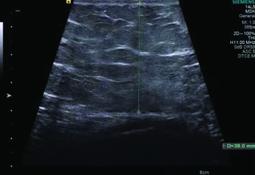
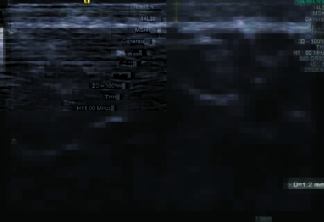
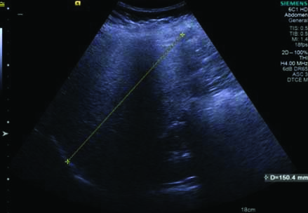
The patients were then subjected to USG using Siemens Acuson S2000 diagnostic ultrasound system (Siemens Healthcare, Erlangen, Germany) with transducers of 3.5-5 MHz, 4-9 MHz and 5-14 MHz frequencies for liver span, SAFT and ST measurements, respectively. SAFT and ST were measured with linear transducer below the umbilicus in the midline, kept at a distance equal to the length of transducer footprint (approx. 2 inches) [Table/Fig-1,2]. The depth of the scan was adjusted according to the best possible view for adequate measurement. The transducer was kept lightly over the skin and measurements were done at end-expiration phase to prevent the compression of abdominal fat layer. The subcutaneous fat was measured as vertical distance from the inferior margin of skin to the linea alba, with the transducer in transverse position. The liver span was measured in the mid-clavicular line cranio-caudally [Table/Fig-3]. All the examinations were done by the same radiologist blinded to the BMI value of the patient.
Greyscale USG image with linear transducer showing the method of measurement of subcutaneous abdominal fat thickness.
Greyscale USG image with linear transducer showing the method of measurement of skin thickness.
Greyscale USG image with convex transducer showing the method of measurement of liver span.
Statistical Analysis
The biophysical and sonographic data was stored in spreadsheets using Microsoft Excel 2010 (Microsoft Corp., Redmond, WA, USA). All statistical analysis was done using SPSS statistics software for Windows, (Version 23.0. Armonk, NY: IBM Corp.) Normality of the variables was tested using the Kolmogorov-Smirnov test. Means of the test variables were compared for statistical significance using one-way ANOVA test. Post-hoc intergroup significance was assessed using Tukey’s-Honest Significant Difference (HSD) test. Receiver Operative Characteristics (ROC) curves were used to determine the best possible sensitivity and specificity of study variables for classifying obese and non obese patients. Pearson’s correlation was used to assess the relationship between different variables and their correlation with BMI. The level of statistical significance was determined at p-value≤0.05.
Results
Total 406 participants were divided into four categories according to the BMI based classification as shown in [Table/Fig-4]. Of these, 54 had BMI≥30 kg/m2 and belonged to the obese category while rest of the 352 patients were under non obese and other three categories i.e., underweight, normal and overweight. Eight cases, all females, were morbidly obese with BMI ranging from 35 to 40 kg/m2. Mean age ranged from 34 to 36 years in all these four categories. Mean values of SAFT and ST showed statistically significant results, as determined by one-way ANOVA [F (3,402)=71.97, p<0.001] and [F (3,402)=4.812, p=0.003] for SAFT and ST respectively. The data highlights increase in the values of these parameters with increasing obesity. Liver span also showed statistical significance in various BMI categories.
Descriptive statistics of total and different BMI category patients.
| Variables | Total (n=406) | Underweight (n=61) | Normal (n=199) | Overweight (n=92) | Obese (n=54) | p-value# |
|---|
| Age (years), mean (SD) | 35 (15) | 34 (18) | 34 (15) | 36 (12) | 36 (15) | 0.811 |
| BMI (kg/m2), mean (SD) | 23.66 (5.20) | 16.85 (1.48) | 21.62 (1.72) | 27.25 (1.38) | 32.76 (3.71) | <0.001* |
| Skin thickness (mm), mean (SD) | 1.21 (0.32) | 1.16 (0.35) | 1.19 (0.30) | 1.22 (0.27) | 1.36 (0.37) | 0.003* |
| Abdominal fat thickness (mm), mean (SD) | 16.00 (8.0) | 8.80 (5.05) | 13.80 (6.17) | 20.78 (6.26) | 23.33 (9.06) | <0.001* |
| Liver span (cm), mean (SD) | 14.10 (1.70) | 13.10 (1.48) | 13.77 (1.47) | 14.75 (1.60) | 15.38 (1.78) | <0.001* |
| Liver echotexture, median (range) | 0 (0-4) | 0 (0-4) | 0 (0-4) | 0 (0-4) | 0 (0-4) | NA |
SD: Standard deviation, NA: Not applied, BMI: Body mass index
#Comparison using ANOVA test; *p-value<0.05
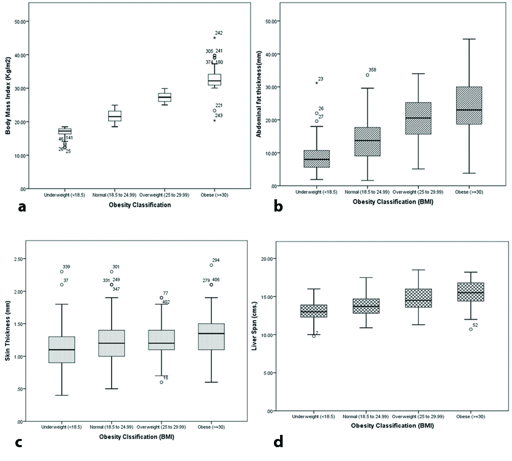
Box-and-whiskers plots [Table/Fig-5a-d] for all the variables showed least overlapping of the IQR for SAFT and was approaching the ideal plot for BMI. SAFT showed significantly higher median value for the overweight and obese categories as compared to the plots for ST and for liver span. Plots in [Table/Fig-5c,d] also show increasing trend with increasing BMI categories; however, showed considerable overlapping in their IQR.
Box and whiskers plots showing distribution of test variables among different classes of BMI. a) ideal box plot showing BMI distribution; b-d) showing distribution of sonographic variables across various BMI based categories. The interior line represents the median, the edges of the box are the upper and lower quartiles (25th and 75th percentile) and the bars (whiskers) display the maximum and minimum values (within 1.5* interquartile range, IQR). There were few outliers.
[Table/Fig-6] shows ROC curves for these parameters with their corresponding best possible predictive values in tabulated form. The SAFT showed highest Area Under the Curve (AUC) with 79% sensitivity and 72% specificity for prediction of obesity (BMI ≥30 kg/m2) at a value of 18.65 mm.
ROC curves of sonographic variables with table showing ROC derived cut off values and their corresponding sensitivity and specificity in classification of obese and non obese.
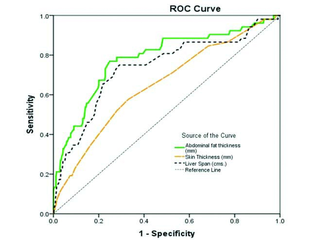 |
| Test Variables | AUC | Cut off value | Sensitivity | Specificity |
| Abdominal fat thickness (mm) | 0.782 | 18.65 | 78.8% | 72% |
| Abdominal skin thickness (mm) | 0.650 | 1.0 | 84.6% | 32% |
| Liver span (cm) | 0.763 | 14.75 | 73% | 73% |
Correlation between the sonographic parameters and BMI was found to be strong and positive for all the variables, suggesting their role in prediction and classification of obese categories; however with less sensitivity and specificity. SAFT again showed the strongest correlation with increasing BMI (r-value=0.627) [Table/Fig-7].
Correlations matrix between variables/markers of obesity.
| Variables | Body mass index (kg/m2) | Abdominal fat thickness (mm) | Abdominal skin thickness (mm) | Liver span (cm) |
|---|
| Body mass index (kg/m2) | r-value | 1 | 0.627** | 0.207** | 0.428** |
| p-value | <0.001 | <0.001 | <0.001 |
| Abdominal fat thickness (mm) | r-value | 0.627** | 1 | 0.237** | 0.261** |
| p-value | <0.001 | | <0.001 | <0.001 |
| Abdominal skin thickness (mm) | r-value | 0.207** | 0.237** | 1 | 0.165** |
| p-value | <0.001 | <0.001 | | 0.001 |
| Liver span (cm) | r-value | 0.428** | 0.261** | 0.165** | 1 |
| p-value | <0.001 | <0.001 | <0.001 | |
*r-value-Pearson’s correlation coefficient
**Correlation is significant at the 0.01 level (2-tailed).
Discussion
Obesity and its related co-morbidities like diabetes and cardiovascular disease have become a major public health issue and are contributing substantially to disease burden in developed and developing countries alike [16]. India being the second most densely inhabited country in the world is currently undergoing swift epidemiological conversion from under nutrition due to poverty to obesity due to wealth [17]. It has therefore become imperative to correctly diagnose obesity before it starts causing its multitude of problems and to nip the problem in the bud.
Most previous reports have relied on measurement of visceral fat thickness for the diagnosis of obesity. However, since this is difficult to measure especially in patients who are very obese or patients with poor acoustic window due to excessive bowel gases, we included only subcutaneous fat and skin thickness in our study.
Previous studies have also demonstrated higher skin thickness in subjects with higher waist circumference and BMI [18]. As the BMI increases, the skin thickness also increases [19]; however, not much research has been done regarding its correlation with obesity and BMI. In our study we also tried to correlate this easily measurable parameter with BMI.
The prevalence of obesity in our study (as calculated by BMI >25 kg/m2) was 36%. The study conducted by Pradeepa R et al., revealed the prevalence of obesity to be 24.6, 16.6, 11.8 and 31.3% in the states of Tamil Nadu, Maharashtra, Jharkhand and Chandigarh respectively [20]. Our study found the prevalence of obesity to be comparable to Chandigarh probably because our study was also conducted in an urban set up. Morbid obesity was seen in only females in our study, possibly due to their sedentary lifestyle in an urban setup. Misra A et al., found the prevalence of obesity to be 15.6% in females and 13.3% in males which was lower than that found in the present study due to different population subset (urban slums) [21].
Our study showed strong positive correlation between BMI and SAFT. Similar results have been achieved in previous studies which have shown that USG measure of subcutaneous adipose tissue in the abdomen increased significantly with body fat percentage in both men and women [22]. Other studies have also used USG to predict the body density of lean men, women, and obese adults [23-25]. A previous study have also found that SAFT of diabetic patients is higher compared to healthy persons which may be associated with higher amount of adipose tissue due to insulin resistance in type 2 diabetes [18]. In people at low to high risk of diabetes or with proven diabetes, SAFT has been associated with increased cardiovascular risk, independent of overall obesity [26]. Higher SAFT has been found to be linked with higher total and LDL cholesterol levels and lower HDL cholesterol levels [26]. It is also reported that subcutaneous fat may have an antiatherogenic effect [27]. However, further studies are definitely needed to establish the same, whereby SAFT measurement might have another role altogether. The evaluation of obesity related co-morbidities was out of the scope of this study. A previous study had also used visceral abdominal thickness for evaluation of obesity and its related comorbidities [5]. However, in the present study this parameter was excluded as its measurement is limited by bowel gases and compromised acoustic window, especially in obese.
Among SAFT, ST and liver span, SAFT was found to be the best to categorise and diagnose obesity. Best cut off value of SAFT for obese (BMI>30 kg/m2) was found to be 18.5 mm. SAFT was found to be the most sensitive and specific for diagnosis of obesity among all the variables. Mean values of SAFT in the present study was 20.78 mm in overweight individuals (BMI values more than 25 and less than 30 kg/m2) and 23.33 mm in obese (BMI more than 30 kg/m2). Akkus O et al., [18] had determined SAFT to be 13.84±8.64 mm in obese males and 22.45±8.12 in obese females and skin thickness to be 2.39±0.52 mm in obese males and 2.35±0.43 mm in obese females. The present study found strong positive correlation between SAFT, ST and liver span among themselves, indicating their ability to be further used in similar studies.
Since, the mean values of SAFT and ST showed statistically significant results in the form of increasing trend with increasing obesity, we propose that they might be used as markers of obesity. Being easy and accurate measures, these parameters will give a good quantitative measure of obesity. Liver span also showed positive correlation with obesity; however, it cannot be used as a marker because of multiple common infections and metabolic diseases affecting the liver span. Reproducibility of USG measurements has been found to be satisfactory in previous studies as indicated by the relatively low intra and interobserver errors [15].
Limitation
The limitation of this study was that we did not categorise obesity in various classes according to SAFT and ST values like BMI. The measurements in a single patient were done by a single radiologist thus, precluding the interobserver variation assessment in this study.
Conclusion
Obesity being a complex disease with multiple aetiological factors, large sample size is required to identify the effects of precise genetic and environmental factors and their relations. The addition of exact and perfect measurements greatly increases the statistical supremacy of studies to identify the cause of obesity and its probable treatment aspects. This study has shown that USG is an excellent modality for the assessment of abdominal SAFT and ST. Addition of USG parameters will significantly enhance the prediction of obesity and can be used as a complimentary method to BMI. This will ultimately help in bracing ourselves to tackle the menace of obesity and its associated diseases.
SD: Standard deviation, NA: Not applied, BMI: Body mass index
#Comparison using ANOVA test; *p-value<0.05
*r-value-Pearson’s correlation coefficient
**Correlation is significant at the 0.01 level (2-tailed).