Introduction
Risk prediction is used widely to model multiple predictors of an event or disease in epidemiology. Time to event is often considered as an outcome of interest in case of modelling risk. Time-to-event is a clinical course duration variable in which the time is calculated as to extend from the time-point when a subject is enrolled in the study or when the treatment begins to the end-point when the event of interest occurs [1]. The event may be adverse (death oroccurence of a disease), positive (conception or discharge from hospital) [2]. Survival data is a commonly encountered time to event data in which at the end of the follow up period the event will probably not have occurred for all study participants. [2] The distinguishing feature of survival data is censoring. Censoring is considered to be present when information on time to outcome event is not available. This occurs when there is loss to follow up or non-occurrence of the outcome event during the period of observation or before the end of a trial (right censoring); or patient had been at risk for disease for a period before entering the study (left censoring); or when the assessment of monitoring is done at a periodical frequency and time to event is known only up to a time interval (interval censoring) [3].
In survival data, the probability of surviving or not experiencing an event in a given length of time is popularly plotted in Kaplan-Meier Survival curve. For this analysis, it is assumed that at any time-point patients who are censored and patients who continue to be followed have same survival prospects [4]. In the Kaplan-Meier (KM) analysis, the KM estimate is computed by considering time in many small intervals and computing the probability of occurrence of an event at the end of each such interval and multiplying these successive probabilities by earlier computed probabilities [4]. Log rank test is a statistical hypothesis test that is used to compare two survival curves and to identify whether there is any difference between the survival times of different groups. However, it does not take into account other explanatory variables [5].
Cox’s proportional hazard model helps to solve this problem and is analogous to multiple regression in this respect. In Cox model, to address for censoring, the time that has elapsed between the start of observation or origin and the outcome event, is modelled as a function of different explanatory factors. The Cox model is a flexible semi-parametric proportional hazard model independent of time in view of the fact that there is no assumption for the form of baseline hazard; but the covariates enter the model linearly [6,7]. In the Cox model the intercept changes with time and information regarding length of time is taken into account.
The model can be expressed as:
log hi(t) = α(t) + β1xi1+ β2xi2 + … + Βkxik
where, α(t) is the unspecified baseline hazard function that can take any form but cannot be negative, and β1 to βk are coefficients of linearly entered covariates [7].
The Cox model is a more generalized form of the Poisson model used for count of events as outcomes in view of the concept that the later can be derived from the former if the baseline hazard (the risk of an individual at baseline before the emergence of explanatory or risk factor of interest) is constant over time. [8] Both the Poisson and Cox regression models assume the hazards to be proportional for individuals with different values of the explanatory variables. Thus, for the model to be used in epidemiologic studies, data must meet the assumptions that the hazards are proportional and that the effect of a given covariate is linear and does not change over time [5].
The Cox model, therefore, in its simplest form fail to explain data related to non-linear effects of covariates and when there are recurrent time-to-event outcomes. The former situation can happen when the hazard function takes the shape of a Gompertzian function (tumour size is slowest at the start and end of a time period and the growth curve approaches right hand asymptote slower than the left hand asymptote), Weibull function (heart attack, in which failure rate is proportional to a power of time) or convex shape (lung cancer) [6,8].
The second important challenge in survival data analysis is handling ordered and/or clustered data. While the former is related to stochastic processes having Markov property, often encountered while studying relapse or recurrence of a disease or condition, clustering is found to be present in case when outcomes in two or more subjects are correlated or more than one outcome within a single subject are aggregated. For example, members of a family shares similar diet and lifestyle, and therefore survival time of the members of the family tends to be associated [9].
In the above-mentioned situations, the classical Cox proportional hazard model cannot be used; and either the classical Cox model needs to be extended further or specialized models should be used to describe the data. In a simulation study to investigate the performance of various regression models using information regarding the time to each recurrent event, it has been shown that the amount of bias encountered following application of various extended Cox models vary substantially and in the absence of known underlying pathology for recurrence, none is better than the Generalized Estimating Equation (GEE)-poisson model [10]. This finding, nevertheless, puts forth the importance of applying specific model for a specific situation.
In this article, we have done a review of different techniques including extensions of the simple Cox model and other statistical modelling techniques using examples related to the field of public health, so that the problem of model misspecification can be curbed in the practice of reporting results to answer the question as to what model is appropriate for analyzing single or recurrent time to event data. Findings were synthesized from literatures retrieved from searches of Pubmed, Embase, Google Scholar, hand searches and authoritative texts. Keywords for search included “Survival Data”, “Survival Analysis”, “Cox Model”, “Proportional Hazard”, “Accelerated Failure Time”, “Extended Cox Models”, “Counting Process Models”, “Recurrent time to event data”, “Marginal Models”, “Cluster Survival Data”, “Ordered Survival Data”, “Multivariate Ordered Failure Time”, “Multistate Model”, “Competing Risk”, “Joint Model”, and “Copula”.
Stratified Cox Model
When the proportional hazard assumption is not satisfied for a particular covariate, a simple solution is to use stratified Cox model. In this model data are stratified into subgroups or strata and Cox model is applied for each subgroup or stratum. The model is given by,
hig(t) = h0g(t) exp(β´xig),
where, g represents the stratum [11].
This technique is particularly useful in the presence of categorical predictors, which are not of direct interest, causing non-proportionality [11].
However, a limitation of this method has been described in the context of a typical two-treatment randomized clinical trial having a time-to-event endpoint, and randomization is stratified by a categorical prognostic factor (for example, gender) [12]. While in such studies it is often assumed that treatment hazard ratio is constant across strata, the use of stratified Cox model may be a risky approach because the said assumption is often subjected to violation. An alternative approach in such case may follow two stages: firstly, the un-stratified Cox regression is run within each stratum and stratum specific log(HR)s are obtained and then they are combined using either sample size or “minimum risk” stratum weight to obtain an overall estimate of the treatment effect [12].
Accelerated Failure Time Model
The proportional hazard model concentrates on the hazard ratio. In clinical trials, however, the hazard ratio depends on length of patient follow up; and therefore, the estimate of hazard ratio is questionable [13]. The difference in median time to event and finding out the confidence interval may be a reasonable estimate [13]. The Accelerated Failure Time (AFT) approach models survival times directly [14]. Estimates of the ratio of the median time to event between treatments are directly available from these models [13]. In AFT models the covariate effects are assumed to be constant and multiplicative over the time scale. This multiplicative effect is modelled by an acceleration factor, which represents the ratio of survival times corresponding to any fixed value of survival time [11]. The semi-parametric AFT model similar to semi-parametric proportional hazard model, like the Cox model, takes into account the censoring.
The univariate form of the semi-parametric AFT model is given by,
Ti = XiTβ + εi, i = 1, …, n;
Where, Ti, Ci and Xi are the log-transformed failure time, censoring time and the p × 1 covariate vector for the ith subject.
The corresponding multivariate AFT model for a random sample of n independent clusters with Ki margin in the ith cluster is given by,
Tik = XikTβ + εik, i = 1, …, n and k = 1, …, Ki [15].
Extension of Cox Models
When the proportional hazard assumption for censored survival data is violated in the sense that covariate processes have a proportional effect on the intensity process of a multivariate count data rather than having a proportional effect on the hazard function, a counting process model is particularly useful [16]. The intensity is the instantaneous conditional failure rate at time t, which is conditional on the occurrence of particular count of set of events till that time.
This model can be used for multivariate ordered failure event type data. In this model each study participant is considered to contribute to the risk set till she/he remains under observation at the time, the event occurs and shares the same baseline hazard function [17].
The Anderson Gill Counting Process (AG-CP) model is a regression analysis of the intensity of a recurrent event and takes into account complicated censoring patterns and time-dependent covariates [16]. The model is given by:
λι(t) = λ0(t)eβ’0Zι(t)Yι(t), I = 1, …, n,
where, β´(t) is the coefficient of time varying explanatory factor Zι(t). Yι(t) denotes the weight process; that is the transition from one state to another of a condition that follows Markov model. In such model the patients are considered to be in a discrete state of health, and the events represent the transition from one state to another. For example, “not admitted” to “admitted” in case of hospital admission process etc. λ0(t) is the baseline intensity of jump from one state to another of the Markov process event; where, intensity refers to the force of change from one state to another [16]. The intensity of jump depends on an unknown nuisance parameter that describes the jump proneness, which is dependent on time [18]. In simpler terms, this is dependent on time varying covariates. When compared with non-survival approaches, like poisson and negative binomial regression, the Anderson Gill approach is comparable to a negative binomial regression and is superior to poisson model which has an increased type I error rate [19]. When compared with the Cox model, the advantages of this model are: 1) ability to accommodate left censored right-continuous data, 2) account for time-varying covariates, 3) can model multiple events, and 4) can model discontinuous interval of risks [20]. However, this model cannot be used when multiple events occur at a given time, e.g. in a study examining time to side effects of a new medication having multiple side effects. Here, at any given time point more than one side effect can occur. In this case, if a patient exhibits two side effects at a given time, one is not considered in the AG-CP model because it assumes the interval between two side effects as zero.
Conditional models are required when a subject is assumed not to be at risk for a subsequent event until a current event has terminated [17]. This means that considering a person at risk for (k+1)th event is conditional on the occurrence of kth event. These models is extension of the counting process model of AG-CP [22]. In this case either the actual time when the event occurs is used after stratifying event by failure order (Prentice, Williams, and Paterson-Conditional Probability model: PWP-CP) or time since the last event is considered assuming that all events start at the time of study entry (Prentice, Williams, and Paterson- Gap Time model: PWP-GT) [17]. In the PWP model, two models are considered in relation to the time scale: PWP- T model (this model measures from the entry time- total time model) and PWP- G model (the model resets the clock at every recurrence- the gap time model) [10]. Thus the fundamental difference between the counting process model and conditional model is that the latter uses event specific baseline hazard for a particular event, while the former models a common baseline hazard for all events. If an overall effect is of interest, counting process model is more suitable, while conditional models are more suitable for the relationship between first event and subsequent event. An advantage of conditional models is that they use sandwich robust standard error technique that can provide estimate even if underlying model is incorrect, particularly in case of time dependent covariates [21]. However, none of these methods can generate unbiased parameter estimates when independent increment assumption is violated [19]. This occurs when there are heteroscedasticity over time and correlation of observations within subjects [22]. In such situation Generalized Estimating Equation (GEE) can be rational alternative [22].
Marginal Models
Marginal models are typically used for clustered survival data. In a recurrent event survival data, for example, in case of modelling of recurrent heart attack in subjects with specific risk factors, measurement at different time point within a subject is possibly correlated, if we suppose that the subsequent occurrence of heart attacks has been accrued by the first event. In such case, the question is often focused on the effect of time and time varying covariates on response variable. GEE model is a marginal model that is particularly useful when there is correlated response. This means GEE can handle multiple observations at multiple fixed time point for each individual in a study. For example, GEE can be used to find out effect of an intervention to reduce proportion of kids with high systolic blood pressure in an American Heart Association 8-week school-programme [23]. Here, three visits are conducted (at baseline, eight weeks follow up and one year post intervention) to answer the study question. The observations of blood pressure at the three visits are correlated for each individual. The advantage of GEE is that it allows for dependence within clusters [21,24]. A plausible example can be to examine how the onset of Diabetes affects the time to blindness, in a study with the primary objective of ascertaining whether laser photocoagulation delays the occurrence of blindness. The dependence between right and left eyes can be addressed with a model similar to GEE with robust standard error estimator [25,26]. In this model the within subject correlation structure is addressed as nuisance parameter [21]. The GEE approach can be generalized for multivariate AFT modelling that accounts for multivariate dependence through working correlation structures to improve efficiency [15]. However, GEE is a population average model, which is a specific form of marginal model. In marginal models, individual heterogeneity is integrated to compute a marginal mean, which is considered as the population average, when the random sample is representative of the population, which is often difficult to obtain in longitudinal studies [27]. Moreover, using a conditional model provides the advantage of estimating individual effect; which is not possible from a population average model [27,28]. This means when longitudinal data is truncated by death, unconditional model f(Yi) reflects only averaging f(Yi|Si) over the survival function f(Si) [29]. Fully conditional models are however different in the sense that they stratify the longitudinal response trajectory by time of death [29]. However, advantage of using GEE is that it can establish a connection between conditional and population average models in case of Generalized Linear Model (GLM) class of outcomes. By estimating the marginal moments from conditional moments GEE can be solved when the random effects have a Gausian distribution [30].
For ordered failure time data or unordered failure time data with different type of event, another marginal model analogous to GEE has been proposed that is known as Wei Lin Weissfeld (WLW) model [31]. Such failure time data can arise when each study participant can potentially experience several events (e.g. infections after surgery) or there is some natural or artificial clustering (example of diabetes retinopathy study provided before) [31]. An excellent example of such situation can be seen in a study analyzing time to first incident detection of several different types of Human Papilloma virus (HPV), in which the Cox model does not address possible correlations between incident HPV infections. WLW model can be used in this case to investigate time to first incident detection of several types of HPV either in the same or different clinical visits, taking into account possible correlations between the types. An overall exposure effect can be modeled in this method even after accounting for different baseline hazard function for each HPV type [32]. The marginal Cox model for jth event in ith clustered can be modelled by:
λj(t;Zij) = λ0eβ’jZij(t), j = 1, …, J; i = 1, …, n
The WLW model estimates the coefficients using maximum partial likelihood and uses a robust sandwich covariance matrix estimate to account for the dependence in multiple failure time [31]. Sandwich estimator is a particularly useful technique to estimate the variance of maximum likelihood estimate when the underlying model is incorrect [33]. This form of marginal model has been proposed as superior to previously postulated Buckley-James method, which uses the usual least square adapted for censoring [34]. The Buckley James estimator was previously used to accommodate censored data in the original GEE approach [35].
Frailty and Shared Frailty Models
A frailty model is particularly useful to model heterogeneity among individuals [36]. In standard survival models it is assumed that all individuals are exposed to same risk and thus the models assume homogeneity. Models that include covariates take into account the observed sources of heterogeneity [37]. However, frailty model has the advantage of incorporating unobserved heterogeneity in addition to observed covariates [38]. It is a random effects model for time variables, where the random effect has a multiplicative effect on the hazard [39]. Here, the hazard function depends upon an unobservable random variable. Even after controlling for different known risk factors, subjects are exposed to different risk levels due to some unobserved covariates and this is modeled in frailty model and is known as frailty [21]. Shared frailty model is particularly useful for multivariate survival data [36].
A simple frailty model can be written as [31]:
hij(t) = h0(t)exp(βTZij(t) + νi)
where, h0(t) is the unspecified baseline hazard and β is the regression coefficient.
The likelihood of the observed data is calculated as a function of this hazard. As the distribution is unknown very often, the best way to find the right distribution is to fit several frailty models with different distributions for baseline hazard [31]. The standard assumption is to use a gamma distribution for the frailty. However, this condition is particularly useful for late events [39]. To identify heterogeneity of a frailty distribution hypothesis test have been proposed considering h0 that yt have a common variance. In this regard, the useful of cusum of squares test has been proposed to detect a variance change and the location of change [40].
Compared to the models discussed above frailty model has much wider applicability, including multivariate (dependent) failure times generated as conditionally independent times given the frailty [39]. However, a major limitation of shared frailty model is that it cannot account for two heterogeneous but independent processes [41]. Such situation may arise in case of chronic diseases like cancer or disease relapses, where a joint analysis of recurrence and mortality processes are needed. In such cases a joint model with correlated frailty may help [41].
Competing Risk and Multistate Models
In simple terms, survival models are two state models in which transition from one state to another is taken into account. Therefore, special techniques are needed when there are more than one state and/ or more than one transition. Such situation may arise in several demographic processes including migration, changes in marital status, in which it becomes necessary to account for the transitions people experience in their life course. These processes are best accounted by multistate models (semi-Markov model). In these models the basic parameters are transition hazard rates or intensities which depend on time spend on a particular state and observed covariates [42]. Several multistate modelling techniques have been developed. Among these some commonly used techniques are:
Competing Risks Model
In Markov process, there are some states for which it is not possible to transition out of the state. These are absorbing states. The remaining ones are transient states [43]. In survival data there are two states: one absorbing state (death) and one transient (alive) state. But for competing risks data there are multiple absorbing states (failure from each of several causes) [43]. Competing risk refers to experience by a patient an event different from the event of interest. For example, in order to determine the incidence of death due to breast cancer among breast cancer patients, death due to some unrelated cause may be a competing risk [44]. While the censoring, usually encountered in survival data is the noninformative censoring, in competing risk data informative censoring from competing risk (for example, death due to causes other than the cause of interest) is also present. In such case, non-parametric estimation of the cumulative incidence by differentiating between the informative and non-informative censoring will help to measure effect of interest. The step-by-step approach of such differentiation has been given by Satagopan JM et al., [44].
Different Multistate Models
The model assumptions for multistate models vary with respect to different type of time dependence of the transition rate from one state to another and presence of intermediate processes. When intensities are constant or independent of time, Time-Homogeneous Markov Models (THMM) are used; when the transition intensities only depend on the history of the process through the current state, non-homogeneous Markov models are used; when future evolution not only depends on the current state h, but also on the entry time th into state h, semi-Markov models are used [45]. However, when the transition intensity depends on the entire path that they took to get to their current state, non-Markov models are used [43]. Therefore, specifying the model depends on assumption regarding Markov process and time-homogeneity. While the assumption regarding the former is checked using Cox Snell Residuals and Akaike’s Information Criterion, the latter is checked by Schoenfeld Residuals [46]. In case of chronic diseases, where the states represent the degree of damage, a progressive Markov process is observed. For example, progression in case of human immunodeficiency virus (HIV) infection: asymptomatic to symptomatic non-Acquired Immunodeficiency Syndrome (AIDS) to AIDS. In such case, the progressive multistate models can provide a convenient framework for reliable parameter estimation [47]. The simplest form of progressive multistate model is transformation the two-state survival model (alive–dead) into progressive three-state model by splitting the alive state into two transient states, which can be generalized to k-progressive model [45]. For HIV infection example, the possible three state model can be: asymptomatic– symptomatic non-AIDS–AIDS. However, application of Cox model for each endpoint separately is not recommended because separate analyses fail to reveal the relationship between different types of events [48]. Parameter estimation using Expectation-Maximization (EM) algorithm and variance estimation using Luis method in case of progressive multistate models have been described in literature [47]. A simple variation of the progressive multistate model is the illness-death model, where illness is an intermediate between disease and death. This is commonly found in oncological studies. For example, in case of cancer patients, post-tumour removal, death can occur in a patient with or without the presence of an intermediate event: isolated loco-regional recurrence [49]. In such case, more general models than Markov models are needed because transition hazards depend on previous state occupation time and presence of two different time scales following the occurrence of the intermediate event: first, the time since entry into the study and second, the time since the occurrence of the intermediate event. In such case, a joint approach has been proposed in the literature [49].
Joint Models
In health services research, outcomes with different attributes, e.g. continuous, count and categorical outcomes are encountered jointly; for example, an adverse health event (binary) can have impact on both length of stay in a hospital and cost [50]. In such case, copula models may be used to link the specified marginal distributions to get a joint distribution for the outcomes [50]. Copula functions enable separate consideration of each variable margin and their dependence structure [51]. In a semi parametric copula model, the probability structure for each failure time is determined marginally, and nonparametric consistent estimators are obtained for marginal survival functions ignoring the dependence. The estimators are then substituted into a conditional likelihood for the association parameter, which yields a pseudo-likelihood and the association parameter is estimated from the pseudo conditional likelihood using estimating equation [52].
Discussion
Semi parametric Cox model is based on proportional hazards assumption, which is often violated. Based on the review of different methods in different situations, we put forward a crude simple algorithm that can serve as a preliminary guideline to prevent model misspecification while analysing survival data [Table/Fig-1]. We recommend the use of stratification in the presence of categorical covariates, for which proportional hazard assumption is violated. However, the number of such covariates should be fewer and a two-staged procedure, discussed above, is often preferable. In case of clinical trials, when follow up periods for various interventions or comparison groups are different, and the Hazard Ratio (HR) depends on follow up period, AFT models are preferred to determine the desired effect in term of acceleration factor. In case of multivariate ordered failure events, when covariates processes have proportional effect intensity process and local martingale assumption is satisfied, the Andersen Gill Counting Process model may be used. However, in the presence of multiple events at each time point in the above case, e.g. multiple side effects of a drug, Prentice Williams Paterson Gap Time Model is used. None of the above mentioned models can be applied in the presence of clustering, for which marginal models, like WLW model may be used. However, marginal models can only provide effect in terms of population average or marginal mean.
Algorithm for model selection in survival data analysis
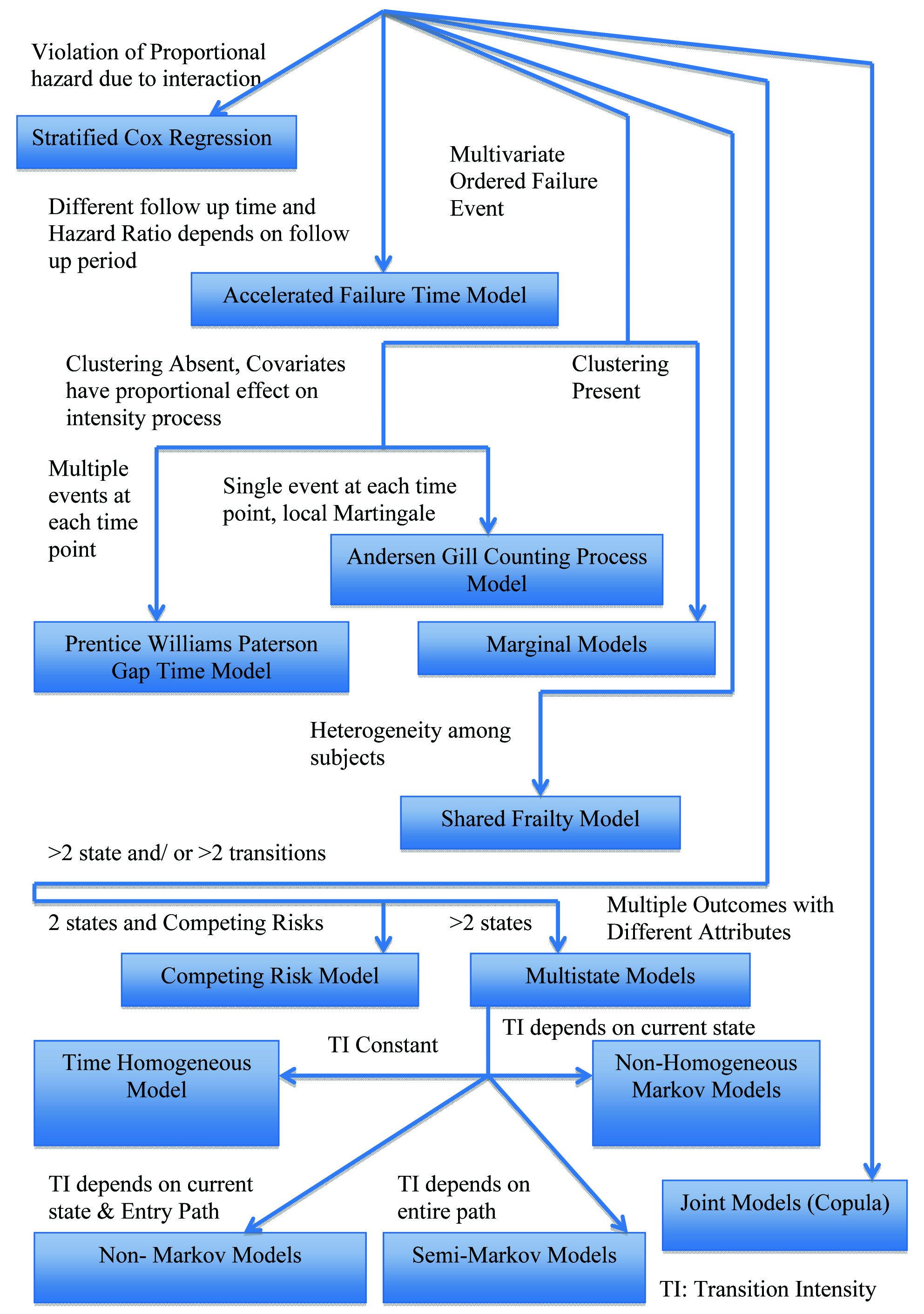
However, GEE can establish a connection between conditional and population average models. But, these models cannot take into account individual heterogeneity, which can be modelled using shared frailty for multivariate data. While all the above-mentioned models are used for two state survival data, they cannot provide reliable parameter estimate in the presence of competing risk(s). In the latter case, a competing risk model may be used. If there are more than two states, however, a multistate model may be used. The choice of model in such case may be determined by the relationship between intensity of transition between states and time scale. In multivariate time to event data, event several different outcomes of different attributes are considered simultaneously, a joint model using copula function can be considered.
Although the method of making choice provided above is crude and subjected to carefully checking assumption of each model before applying, it is expected to aid researchers, especially who are naïve in this field, develop a clear perspective about what model is suitable based on the research question, study design, censoring pattern and underlying dependence among different failure events.
[1]. Rich JT, Neely JG, Paniello RC, Voelker CCJ, Nussenbaum B, Wang EW, A practical guide to understanding Kaplan-Meier curvesOtolaryngol Head Neck Surg 2010 143(3):331-6. [Google Scholar]
[2]. Altman DG, Bland JM, Statistics Notes: Time to event (survival) dataBMJ 1998 317(7156):468-9. [Google Scholar]
[3]. Prinja S, Gupta N, Verma R, Censoring in clinical trials: review of survival analysis techniquesIndian J Community Med 2010 35(2):217-21. [Google Scholar]
[4]. Goel MK, Khanna P, Kishore J, Understanding survival analysis: Kaplan-Meier estimateInt J Ayurveda Res 2010 1(4):274-8. [Google Scholar]
[5]. Bewick V, Cheek L, Ball J, Statistics review 12: Survival analysisCrit Care 2004 8(5):389 [Google Scholar]
[6]. Lin C-Y, Halabi S, On model specification and selection of the Cox proportional hazards modelStat Med 2013 32(26):4609-23. [Google Scholar]
[7]. Fox J, Weisber S, Cox Proportional-Hazards Regression for Survival Data in RIn An Appendix to An R Companion to Applied Regression 2011 :1-20. [Google Scholar]
[8]. Rachet B, Stavola B, De Belot A, Survival AnalysisCentre for Statistical Methodology Seminar 2017 [Google Scholar]
[9]. Cleves M, Gould WW, Gutierrez RG, Marchenko YU, An Introduction to Survival Analysis Using Stata. Second 2008 TexasStata Press:7-19. [Google Scholar]
[10]. Lei N, Flexible Partially Linear Single Index Regression Models for Multivariate Survival DataThe University of Western Ontario 2013 Available from: http://ir.lib.uwo.ca/cgi/viewcontent.cgi?article=3177&context=etd [Google Scholar]
[11]. Mieno MN, Yamaguchi T, Ohashi Y, Alternative statistical methods for estimating efficacy of interferon beta-1b for multiple sclerosis clinical trialsBMC Med Res Methodol 2011 11(1):80 [Google Scholar]
[12]. Qi J, Comparison of Proportional Hazards and Accelerated Failure Time ModelsUniversity of Saskatchewan 2009 Available from: https: //ecommons. usask.ca/bitstream/handle/10388/etd-03302009-140638/JiezhiQiThesis.pdf?sequence=1&isAllowed=y [Google Scholar]
[13]. Mehrotra D V, Su S-C, Li X, An efficient alternative to the stratified Cox model analysisStat Med 2012 31(17):1849-56. [Google Scholar]
[14]. Keene ON, Alternatives to the hazard ratio in summarizing efficacy in time-to-event studies: an example from influenza trialsStat Med 2002 21(23):3687-700. [Google Scholar]
[15]. Swindell WR, Accelerated failure time models provide a useful statistical framework for aging researchExp Gerontol 2009 44(3):190-200. [Google Scholar]
[16]. Chiou SH, Fitting Accelerated Failure Time Models in Routine Survival Analysis with R package aftgeeJ Stat Softw 2014 61(11):1-23. [Google Scholar]
[17]. Andersen PK, Gill RD, Cox’s Regression Model for Counting Processes: A Large Sample StudyAnn Stat 1982 10(4):1100-20. [Google Scholar]
[18]. Guo Z, Gill TM, Allore HG, Modeling repeated time-to-event health conditions with discontinuous risk intervals. An example of a longitudinal study of functional disability among older personsMethods Inf Med 2008 47(2):107-16. [Google Scholar]
[19]. Svensson A, Estimation in some Counting Process Models with Multiplicative StructureAnn Stat 1989 17(4):1501-8. [Google Scholar]
[20]. Jahn-Eimermacher A, Comparison of the Andersen–Gill model with poisson and negative binomial regression on recurrent event dataComput Stat Data Anal 2008 52(11):4989-97. [Google Scholar]
[21]. Johnson CJ, Boyce MS, Schwartz CC, Haroldson MA, Modeling Survival: Application of the Andersen–Gill Model to Yellowstone Grizzly BearsJ Wildl Manage 2004 68(4):966-78. [Google Scholar]
[22]. Sagara I, Giorgi R, Doumbo OK, Piarroux R, Gaudart J, Modelling recurrent events: comparison of statistical models with continuous and discontinuous risk intervals on recurrent malaria episodes dataMalar J 2014 13(1):293 [Google Scholar]
[23]. Shoben AB, Emerson SS, Violations of the independent increment assumption when using generalized estimating equation in longitudinal group sequential trialsStat Med 2014 33(29):5041-56. [Google Scholar]
[24]. Weaver MA, Introduction to Analysis Methods for Longitudinal/ Clustered Data, Part 3: Generalized Estimating EquationsFamily Health International 2009 GoaAvailable from: http://www.icssc.org/Documents/AdvBiosGoa/Tab07.00_GEE.pdf [Google Scholar]
[25]. Hanley JA, Negassa A, Edwardes MD, deB Forrester JE, Statistical Analysis of Correlated Data Using Generalized Estimating Equations: An OrientationAm J Epidemiol 2003 157(4):364-75. [Google Scholar]
[26]. Glynn RJ, Rosner B, Regression methods when the eye is the unit of analysisOphthalmic Epidemiol 2012 19(3):159-65. [Google Scholar]
[27]. Lee Y, Nelder Ja, Conditional and Marginal Models: Another ViewceStatistical Sci 2004 19(2):219-38. [Google Scholar]
[28]. Lindsey JK, Lambert P, On the appropriateness of marginal models for repeated measurements in clinical trialsStat Med 1998 17(4):447-69. [Google Scholar]
[29]. Kurland BF, Johnson LL, Egleston BL, Diehr PH, Longitudinal Data with Follow-up Truncated by Death: Match the Analysis Method to Research AimsStat Sci 2009 24(2):211 [Google Scholar]
[30]. Zeger SL, Liang KY, Albert PS, Models for longitudinal data: A generalized estimating equation approachBiometrics 1988 44(4):1049-60. [Google Scholar]
[31]. Gharibvand L, Liu L, Analysis of Survival Data with Clustered EventsSAS Glob Forum 2009 237:1-11. [Google Scholar]
[32]. Xue X, Gange SJ, Zhong Y, Burk RD, Minkoff H, Massad LS, Marginal and mixed-effects models in the analysis of human papillomavirus natural history dataCancer Epidemiol Biomarkers Prev 2010 19(1):159-69. [Google Scholar]
[33]. Freedman DA, On the So-Called “Huber Sandwich Estimator” and “Robust Standard Errors.”Am Stat 2004 60(4):299-302. [Google Scholar]
[34]. Wei LJ, The accelerated failure time model: A useful alternative to the cox regression model in survival analysisStat Med 1992 11(14–15):1871-9. [Google Scholar]
[35]. Hornsteiner U, Hamerle A, A Combined GEE/Buckley-James Method for Estimating an Accelerated Failure Time Model of Multivariate Failure TimesSonderforschungsbereich 1996 386 [Google Scholar]
[36]. Gutierrez RG, Parametric frailty and shared frailty survival modelsStata J 2010 10(3):288-308. [Google Scholar]
[37]. Rodrıguez G, Unobserved HeterogeneityHandouts for ‘Pop509: Survival 2005 Available from: http://data.princeton.edu/pop509/UnobservedHeterogeneity.pdf [Google Scholar]
[38]. Yashin AI, Iachine IA, Begun AZ, Vaupel JW, HIDDEN FRAILTY: MYTHS AND REALITY [Google Scholar]
[39]. Hougaard P, Frailty models for survival dataLifetime Data Anal 1995 1(3):255-73. [Google Scholar]
[40]. Taylor P, Lee S, Lee S, Communications in Statistics - Theory and Methods Testing Heterogeneity for Frailty Distribution in Shared Frailty Model 2006 2014 :37-41. [Google Scholar]
[41]. Belot A, Rondeau V, Remontet L, Giorgi R, CENSUR working survival groupA joint frailty model to estimate the recurrence process and the disease-specific mortality process without needing the cause of deathStat Med 2014 33(18):3147-66. [Google Scholar]
[42]. Bijwaard GE, Unobserved Heterogeneity in Multiple-Spell Multiple-States Duration ModelsIZA Discuss Pap Ser 2011 (5748) [Google Scholar]
[43]. Logan BR, Review of multistate models in hematopoietic cell transplantation studiesBiol Blood Marrow Transplant 2013 19(1 Suppl):S84-7. [Google Scholar]
[44]. Satagopan JM, Ben-Porat L, Berwick M, Robson M, Kutler D, Auerbach AD, A note on competing risks in survival data analysisBr J Cancer 2004 91(7):1229-35. [Google Scholar]
[45]. Meira-Machado L, de Uña-Alvarez J, Cadarso-Suárez C, Andersen PK, Multi-state models for the analysis of time-to-event dataStat Methods Med Res 2009 18(2):195-222. [Google Scholar]
[46]. Ali Z, Mahmood M, Kazem M, Hojjat Z, Mostafa H, Kourosh HN, Assessing Markov and time homogeneity assumptions in multi-state models: application in patients with gastric cancer undergoing surgery in the Iran cancer instituteAsian Pac J Cancer Prev 2014 5(1):441-7. [Google Scholar]
[47]. Chen B, Yi GY, Cook RJ, Progressive multi-state models for informatively incomplete longitudinal dataJ Stat Plan Inference 2011 141(1):80-93. [Google Scholar]
[48]. Putter H, van der Hage J, de Bock GH, Elgalta R, van de Velde CJH, Estimation and prediction in a multi-state model for breast cancerBiom J 2006 48(3):366-80. [Google Scholar]
[49]. Meier-Hirmer C, Schumacher M, Multi-state model for studying an intermediate event using time-dependent covariates: application to breast cancerBMC Med Res Methodol 2013 13(1):80 [Google Scholar]
[50]. Gardiner JC, Joint Modeling of Mixed Outcomes in Health Services Research 2013. (SAS Global Forum). Report No. 435 2013 [Google Scholar]
[51]. Murteira JMR, Lourenço ÓD, Health Care Utilization and Self-Assessed Health Specification of Bivariate Models Using CopulasHeal Econom Data Gr Work Papcited 2016 Feb 5Available from: http://ideas.repec.org/p/yor/hectdg/07-27.html [Google Scholar]
[52]. Zhu H, Wang M-C, Analysing bivariate survival data with interval sampling and application to cancer epidemiologyBiometrika 2012 99(2):345-61. [Google Scholar]